Abstract Link to heading
I have recently updated my Pixel 3 to run Android 12 which has brought many new features. The most obvious is the introduction of Material You - Android’s new design language - which comes with (what I think) is a pretty awesome feature that will extract accent colours from your wallpaper to use throughout the system UI. What follows is my attempt to build a similar system that can take an image and create a pallette of accent colours and some interesting outputs along the way!
Menu Link to heading
Accessing Colour Data
Clustering Techniques
Re-drawing Our Image
Determining the Colour Pallette
Accessing Colour Data Link to heading
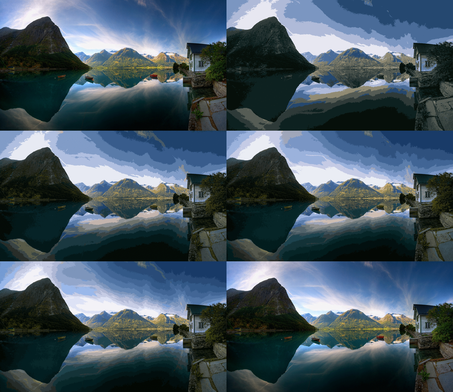
In order to be able to extract colours from an image, we first need to understand how a picture is stored and displayed. There are many different colour models that can be used to represent the colour of an individual pixel within an image, the most common being the RGB model. This has three values, one for each channel relating to Red, Green & Blue. The reason that these colours are used is that they can be “added” together to form many different colours, e.g. mixing blue and red will give shades of pink and purple. We can use the imager package in R to access these values along with an (x, y) co-ordinate to specify the location of a particular pixel. For example take this image of a Norwegian Fjord and subsequent R data for this image:

library(data.table)
library(imager)
## -------------------------------------------------------------------------
## Open image and get pixel colour data ####
img <- dcast(setDT(as.data.frame(load.image("Norway.jpg"))), x + y ~ cc)
colnames(img) <- c("x", "y", "R", "G", "B")| x | y | R | G | B |
|---|---|---|---|---|
| 1 | 1 | 0.435 | 0.560 | 0.760 |
| 1 | 2 | 0.447 | 0.572 | 0.773 |
| 1 | 3 | 0.411 | 0.541 | 0.752 |
| 1 | 4 | 0.458 | 0.580 | 0.835 |
| 1 | 5 | 0.419 | 0.537 | 0.752 |
Here we can see that the first pixel, displayed in the top left corner is represented by 44% red, 56% green and 76% blue. If we take a pixel that is part of the boat just right of centre it has values of 45%, <1% & 2% respectively giving it a dark red colour.
While we see these values as percentages, they are actually stored as numeric values with differing scales depending on what’s known as the bit depth of an image. In this case our image has a bit depth of 24, indicating that 8 bits of data are used to store each colour channel or a value between 0 and 255. This gives us a maximum of 16,777,216 different colours that could be present in an image of this bit depth. On inspection of our image, we have ~140k unique colours displayed. While we could try and extract colours using this full set of information, we will be better served trying to reduce this to a more manageable dataset.
Clustering Techniques Link to heading
The idea of grouping up datapoints based on their similarity or ‘closeness’ to one another is a form of unsupervised learning called clustering. There are plenty of approaches to this, but here we are going to talk about two of the most commonly used - k-means and hierarchical clustering. The goal of both of these is to take our full dataset and assign each datapoint (in our case each pixel of the image) to a group of datapoints that are all closely related to each other.
k-means Link to heading
With k-means, we need to specify the number of groups that we want in our output, denoted by the letter k. Once this has been chosen, let’s use 3 as an example, we select three starting points to become the centrepoint of each of our 3 clusters. Each datapoint is then assigned to the centrepoint that it is closest to, generally using a euclidean distance. In our colour example, this would be calculated as the square root of the sum of squared differences between the R, G & B values of our datapoint and each cluster centre. Once all datapoints have been allocated we then calculate a new cluster centre and repeat this process. We stop once we reach a threshold where the cluster centres are no longer moving.
Talk about k-Means as a clustering technique that can be used to group together many observations and classify them as all sharing similarity. We can manually specify the value of k to extract a specific number of clusters, or in our case a group of similarly coloured pixels. We can represent each of these clusters by the cluster centre, which for us will be the “average” colour (or average red, green & blue channels) of all the pixels in that cluster. Note that this resulting cluster centre may not be present in the original image!
Re-drawing Our Image Link to heading
At this point we’ll go off on a small tangent. I had the idea that we could create these clusters for increasing numbers of k and then “re-draw” the image using only these colours. To do this we can take each pixel in the original image and change it so that it is actually represented by the centre of the cluster it belongs to, rather than the original colour. Animating this then gives some quite pretty and interesting results!

Norway Fjord (k-means)

Norway Fjord (hierarchical)
Determining the Colour Pallette Link to heading
Hello, World!